Comparing sentiment analysis from different lexicon of Pride and Prejudice Novel

Working with text mining means we can dig more about what the content meaning in particular text. We can see the emotional tone that used by the author, it is positive or negative. Thus we can called opinion mining or sentiment analysis.

We know there are several methods to do the sentiment analysis but in this article we want to discuss about sentiment analysis using lexicon in tidytext package. Here are the three different lexicons based on unigrams:

1. AFINN from Finn Årup Nielsen,
2. bing from Bing Liu and collaborators, and
3. nrc from Saif Mohammad and Peter Turney.

The Bing lexicon uses a binary categorization model that sorts words into positive or negative positions.The AFINN lexicon grades words between -5 and 5 (positive scores indicate positive sentiments).The NRC lexicon categorizes sentiment words into positive, negative, anger, anticipation, disgust, fear, joy, sadness, surprise and trust.

So, let’s start the code:

1. import the library

library(tidytext) 
library(janeaustenr) 
library(dplyr)
library(stringr)
library(tidyr)
library(ggplot2) 

2. Use filter() to choose only the words from one novel we are interested. In this case we used Pride and Prejudice by janeaustenr package. Janeaustenr provides text in novel as a one-row-per-line format.

pride_prejudice <- tidy_books %>%
  filter(book == "Pride & Prejudice")

pride_prejudice

(Output)
# A tibble: 122,204 x 4
   book              linenumber chapter word     
   <fct>                  <int>   <int> <chr>    
 1 Pride & Prejudice          1       0 pride    
 2 Pride & Prejudice          1       0 and      
 3 Pride & Prejudice          1       0 prejudice
 4 Pride & Prejudice          3       0 by       
 5 Pride & Prejudice          3       0 jane     
 6 Pride & Prejudice          3       0 austen   
 7 Pride & Prejudice          7       1 chapter  
 8 Pride & Prejudice          7       1 1        
 9 Pride & Prejudice         10       1 it       
10 Pride & Prejudice         10       1 is       
# ... with 122,194 more rows
 

3. Use inner_join() to calculate the sentiment in different ways.

afinn <- pride_prejudice %>% 
  inner_join(get_sentiments("afinn")) %>% 
  group_by(index = linenumber %/% 80) %>% 
  summarise(sentiment = sum(value)) %>% 
  mutate(method = "AFINN")

bing_and_nrc <- bind_rows(
  pride_prejudice %>% 
    inner_join(get_sentiments("bing")) %>%
    mutate(method = "Bing et al."),
  pride_prejudice %>% 
    inner_join(get_sentiments("nrc") %>% 
                 filter(sentiment %in% c("positive", 
                                         "negative"))
    ) %>%
    mutate(method = "NRC")) %>%
  count(method, index = linenumber %/% 80, sentiment) %>%
  pivot_wider(names_from = sentiment,
              values_from = n,
              values_fill = 0) %>% 
  mutate(sentiment = positive - negative) 

The %/% operator does integer division (x %/% y is equivalent to floor(x/y)) so the index keeps track of which 80-line section of text we are counting up negative and positive sentiment in.

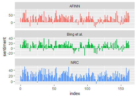
4. We now have an estimate of the net sentiment (positive - negative) in each chunk of the novel text for each sentiment lexicon. Let’s bind them together and visualize them

bind_rows(afinn, 
          bing_and_nrc) %>%
  ggplot(aes(index, sentiment, fill = method)) +
  geom_col(show.legend = FALSE) +
  facet_wrap(~method, ncol = 1, scales = "free_y")

And here is the result:

From the plot, we can see there are a similiarity and also differences among those lexicon. The similiarity is changes of slope of the plot. In other hand, the most significant differences is about the values.

First, the AFINN give highest positive values. It can reach more than 50. Second, NRC has the biggest values of the positive. Last, Bing has the highest negative values.

How this happened? We can trace by the values of positive and negative words in these lexicon:

get_sentiments("nrc") %>% 
  filter(sentiment %in% c("positive", "negative")) %>% 
  count(sentiment)
  
  (Output)
  
  # A tibble: 2 x 2
  sentiment     n
  <chr>     <int>
1 negative   3318
2 positive   2308

gget_sentiments("bing") %>% 
  count(sentiment)
  
  (Output)
  
  # A tibble: 2 x 2
  sentiment     n
  <chr>     <int>
1 negative   4781
2 positive   2005

The bing lexicon has higher values of negative than the NRC. So it will affect the plot visualization and make the plot of Bing has the highest value of negative.

How with AFINN? It is stated before that AFINN lexicon assigns words with a score that runs between -5 and 5, with negative scores indicating negative sentiment and positive scores indicating positive sentiment. Here the result of AFINN lexicon:

afinn
# A tibble: 163 x 3
   index sentiment method
   <dbl>     <dbl> <chr> 
 1     0        29 AFINN 
 2     1         0 AFINN 
 3     2        20 AFINN 
 4     3        30 AFINN 
 5     4        62 AFINN 
 6     5        66 AFINN 
 7     6        60 AFINN 
 8     7        18 AFINN 
 9     8        84 AFINN 
10     9        26 AFINN 
# ... with 153 more rows

This values of differences gave us the information about the important context when choosing the sentiment lexicon for analysis.